
Week 1 - CMB
Week 1 Exercise: Plotting with Matplotlib in Python
If you are already familiar with plotting with matplotlib using python, you will find the following uninteresting, but please make sure that you are familiar with the blackbody physics and plots shown below.
If you get stuck, you can send an email to ostemboard@colorado.edu
In the following exercise, we are going to make sure you are ready for the workshop by plotting several curves. These curves are ideal blackbody spectra. The CMB is one of the most ideal black bodies we have measured to date.
What is a blackbody? It is a perfect absorber of light. That means no light is reflected off its surface. It is also perfectly opaque; no light gets through the blackbody. Most things around you are pretty poor at approximating blackbodies.
The one type of light a blackbody gives off is its emission spectrum. This spectrum is interesting because it is only related to the temperature of the object. That means that if I know the temperature of the object, I can predict its ideal blackbody behavior.
We can thank the physicist Max Plank for doing the math for us and telling us that the spectrum of a blackbody at temperature T is:
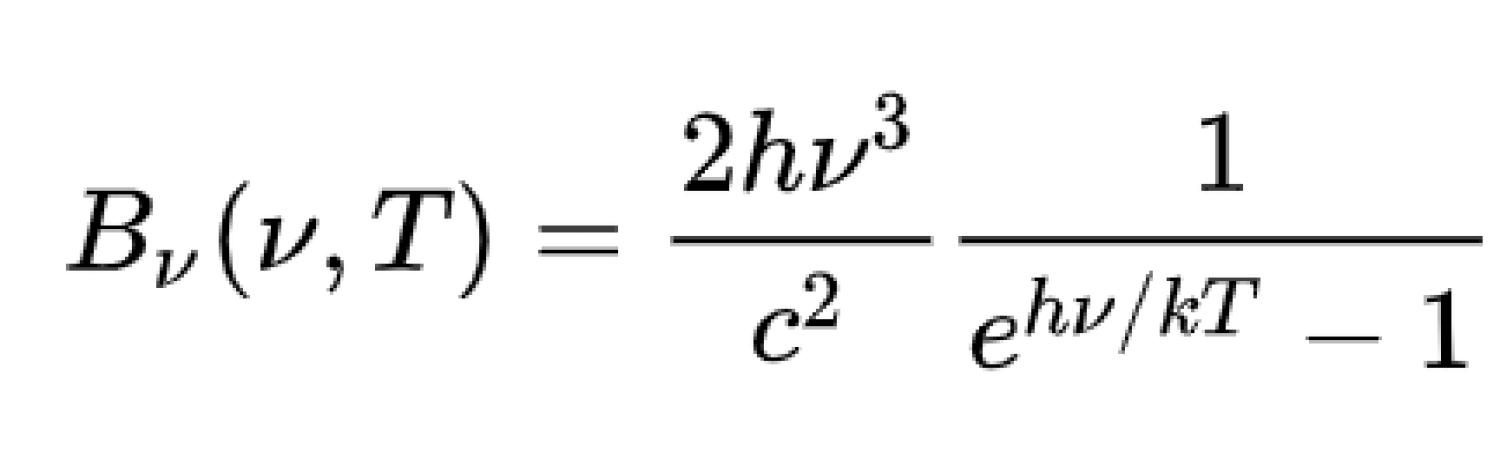
The only real variables here are the frequency nu and the temperature T. Everything else is a constant. h is called Planck’s Constant. c is the speed of light. k is the Boltzmann’s constant. What is remarkable about this equation is that it uses constants from three theories: quantum mechanics (h), relativity (c), and statistical mechanics (k). If you have not taking calculus yet, you might not be familiar with e. e is a number, like pi or 2 or 2345.6. Here, e is raised to the power of h*nu/(k*T).
Alright, so the weirdest thing about this equation is its output: this mysterious B(nu, T). B is called the spectral radiance and it has the absolute worst units that you will have to deal with in physics. These units are: [Watts]/[sr]/[meters]^2/[Hz].
Okay, so [sr] is short for a steradian or a unit of solid angle (a solid angle is a certain percent of the surface of a sphere just as a degree is certain percent of a circle). Watts is the SI unit for power, and this is the real takeaway here. Power is the amount of energy emitted during a period of time; Watts corresponds to the amount of energy emitted in Joules over a period of one second. So when we plot spectral radiance as a function of frequency at a given temperature, we will see the amount of power will change depending on what wavelength we are looking at. Pretend that you had super eyes and could see all wavelengths of light (and could tell what frequency of light was that you were looking at). Then you would see the room temperature iron bar glowing and note that it is glowing mostly in the infrared. But you would also see that the iron bar glowing in the visible spectrum, the x ray spectrum, the radio spectrum, but no where near as bright as in the infrared spectrum.
Okay, now we are ready to plot. Open your preferred IDE (in Anaconda, you can use Spyder) and we can get started.
First, we need to import the matplotlib.pyplot library and the numpy library. We do this by specifying the following:

The nicknames make the libraries easier to work with when we are using functions from those libraries. These nicknames are fairly standard, but you can call them whatever you want:

It will work just fine, but you might forget down the road what ‘potato’ really stands for, so it is best to use names that hint what that library actually contains.
Run the code now (most IDEs have a green arrow). If you get an error, you probably do not have these libraries properly installed.
Okay, now we need to generate some arrays. Let’s write down some interesting temperatures with the following code:

The first temperature is the the temperature of the CMB. The other three temperatures are of stars: Belteguese, the Sun, and Sirius. The units are in Kelvins (K). In order to convert from Celsius to Kelvin, you just add 273. So 0 Celsius is 273 K. In most physics and astronomy research, we are dealing with such extreme temperatures that the boiling point of water is no longer important but the absolute temperatures of objects are. Because of this, we use Kelvins.
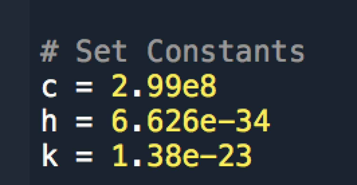
Okay, next I define the constants I will use in SI units. In Python, when I write XeY, where X and Y are numbers, I am actually writing the number X x 10^Y (scientific notation). As an example, 3.4e4 is 34,000 or 34x10^4.
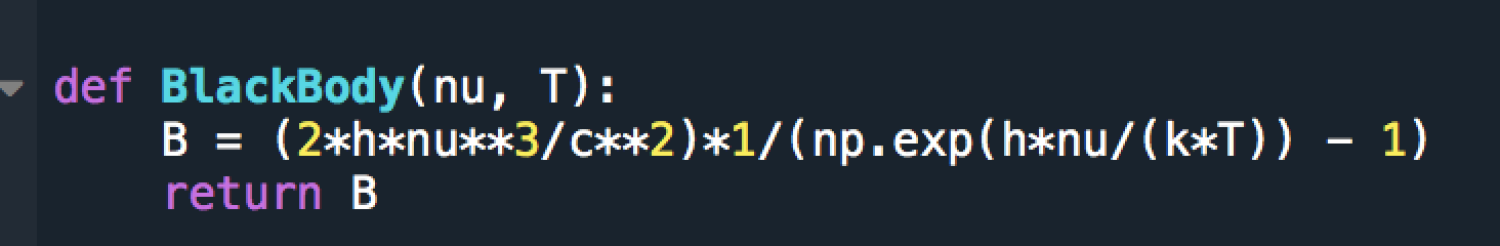
I am going to write a function that will calculate the spectrum for me. The function is called BlackBody and the arguments of the function are nu and T. On the second line, I am assigning the variable B to an algebraic equation. This is the same equation as the blackbody spectrum! On the third line, I state that my function is returning the value B.
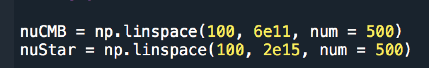
Next, I go ahead and create some arrays. Then, I plot!
I’d like to be able to plot the star blackbody spectra on one plot. Rather than writing it out three times, I can do this with a for loop. A for loop iterates over an object (in this case range(len(temps) - 1)). The length of temps is 4, so len(temps) - 1 is three or three times. I could have written range(3), but this is slightly better because I might want to add more start temps in the future!
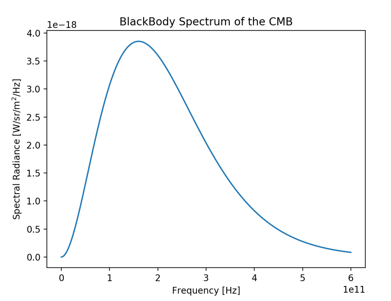
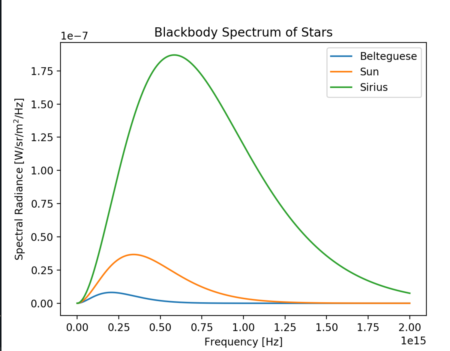
The final plots you should get are shown below.
JUST INCASE your images are not loading, here is the full code:
import numpy as np
import matplotlib.pyplot as plt
temps = np.array([2.725, 3500, 5778, 9940])
# Set Constants
c = 2.99e8
h = 6.626e-34
k = 1.38e-23
def BlackBody(nu, T):
B = (2*h*nu**3/c**2)*1/(np.exp(h*nu/(k*T)) - 1)
return B
nuCMB = np.linspace(100, 6e11, num = 500)
nuStar = np.linspace(100, 2e15, num = 500)
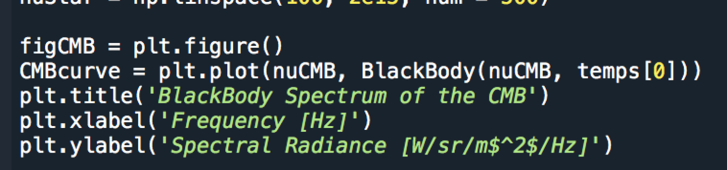
figCMB = plt.figure()
CMBcurve = plt.plot(nuCMB, BlackBody(nuCMB, temps[0]))
plt.title('BlackBody Spectrum of the CMB')
plt.xlabel('Frequency [Hz]')
plt.ylabel('Spectral Radiance [W/sr/m$^2$/Hz]')
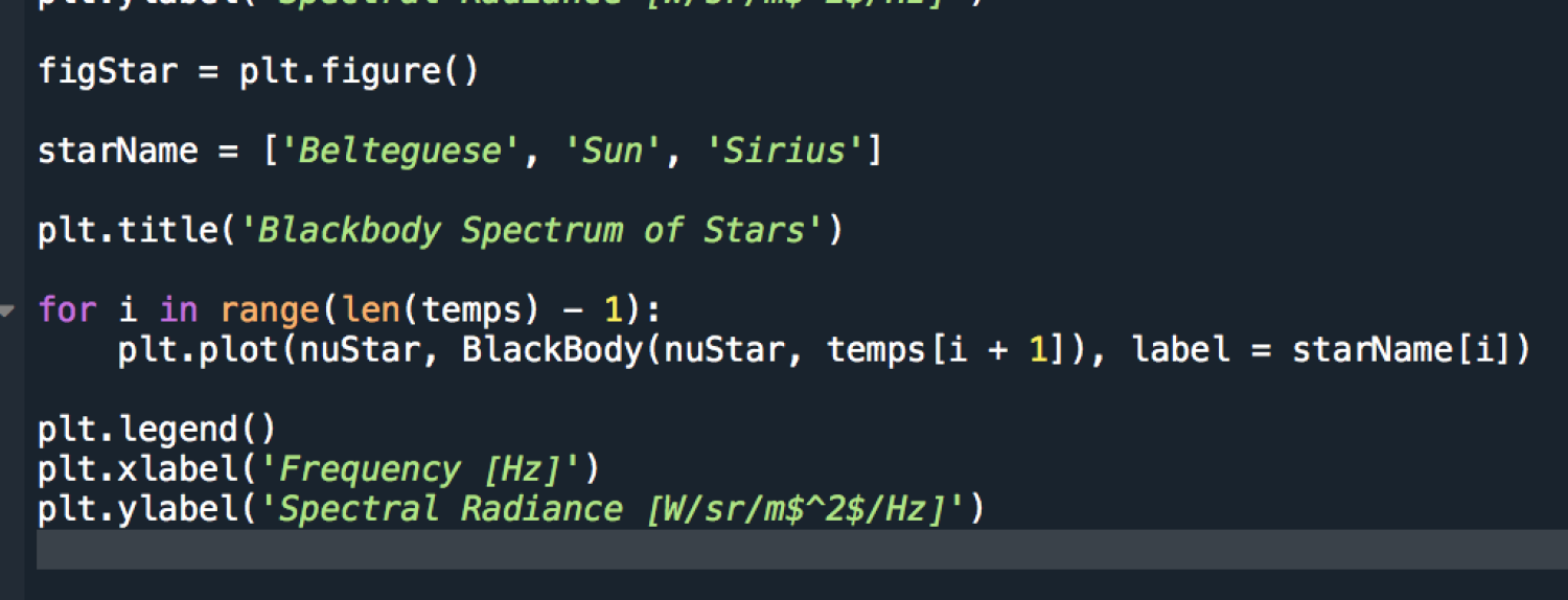
figStar = plt.figure()
starName = ['Belteguese', 'Sun', 'Sirius']
plt.title('Blackbody Spectrum of Stars')
for i in range(len(temps) - 1):
plt.plot(nuStar, BlackBody(nuStar, temps[i + 1]), label = starName[i])
plt.legend()
plt.xlabel('Frequency [Hz]')
plt.ylabel('Spectral Radiance [W/sr/m$^2$/Hz]')