Spatial Statistics in R, Spring 2017
Spatial Statistics in R
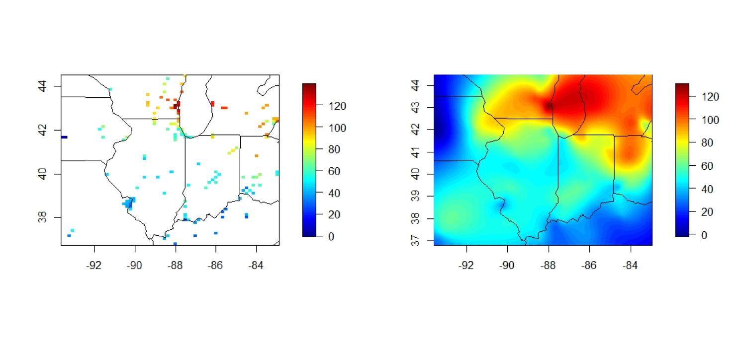
Dealing with an autocorrelated response variable is a frequent problem in regression. Using R, it is easy to visualize and analyze this type of data using spatial statistics. We will discuss the meat of modeling continuously varying spatial data: incorporating relationships between variables based on proximity. This is accomplished by specifying a covariance or variogram model. We will show how to easily visualize your spatial data and estimate its covariance structure. We will then use our specified model to do prediction at new locations. We will provide a brief discussion of the three categories of spatial data sets: point-referenced (continuously varying) data, areal data, and point processes. We will be using the ozone2 data set in the fields package in R, which gives readings of ozone levels at various locations in the US. Participitants are encouraged to follow along in R on their own laptops.
Presenters: Zachary Mullen and Ashton Wiens
Location: Muenzinger E131
Time: Tuesday, March 14, 5:00 - 7:00 PM
Slides:
R Script:
#Clean up my workspace; save my working directory; load packages
setwd("...")
windows()
rm(list=ls())
library(geoR)
library(mapproj)
library(fields)
library(nlme)
#load my test data; have a look
data(COmonthlyMet)
dim(CO.loc)
lonlat<-CO.loc
elev<-CO.elev
temps<-CO.tmax.MAM.climate
#Response variable: CO.tmax.MAM.climate
#Spring seasonal means
#(March, April,May) means by station for the period 1960-1990. If less than 15 years are
#present over this period an NA is recorded. No detreding or other adjustments have been
#made for these mean estimates.
#Visualize!
quilt.plot(lonlat,temps)
US(add=TRUE)
#annoying map problem; change lonlat->dist:
hold <- mapproject(x=lonlat[,1],y=lonlat[,2],projection="sinusoidal")
xy <- cbind(hold$x,hold$y)
#Also annoying: missing values:
hold <- !is.na(temps)
temps <- temps[hold]
elev <- elev[hold]
xy <- xy[hold,]
#Regress
lm1<-lm(temps~xy[,1]*xy[,2]+elev)
summary(lm1)
quilt.plot(xy,lm1$fitted.values)
quilt.plot(xy,lm1$residuals)
savePlot(filename = "Residuals1",type = c("jpg"))
#Make an xy distance matrix
dist.mat<-rdist(xy)
dist.seq<-seq(0,max(dist.mat),length.out=50)
vg<-variog(data=lm1$residuals,coords=xy,breaks=dist.seq)
plot(vg)
par(mfrow=c(1,1))
#eyefit(vg)
#rigorous estimates
vfit<-variofit(vg,cov.model='matern',weights='cressie',nugget=.12,fix.nugget=TRUE )
res.sill<-as.numeric(summary(vfit)$spatial.component[1])
res.range<-as.numeric(summary(vfit)$spatial.component[2])
res.nu<-as.numeric(summary(vfit)$spatial.component.extra[1])
#eyeball estimates
res.sill<-.90; res.nugget<-.12; res.range<-.011; res.nu<-.5
#resestimate the mean using GLS
Sigma<-Matern(dist.mat,nu=res.nu,range=res.range)
lowertri.Sigma<-Sigma[lower.tri(Sigma,diag=FALSE)]
lm2<-gls(temps~xy[,1]*xy[,2]+elev,correlation=corSymm(lowertri.Sigma,fixed=TRUE))
#reestimte spatial structure so we can Krige
vg2<-variog(data=lm2$residuals,coords=xy,breaks=dist.seq)
#eyefit(vg2)
res2.sill<-1.17;res2.nugget<-.3;res2.range<-.022;res2.nu<-1
#That Krige Matrix stuff
Sigma2<-res2.sill*Matern(dist.mat,nu=res2.nu,range=res2.range)
krig<-Sigma2%*%solve(Sigma2+diag(res2.nugget,length(xy[,1])))%*%lm2$residuals
#How did we do
par(mfrow=c(1,3))
quilt.plot(xy,temps,main='Data',zlim=c(0,25))
quilt.plot(xy,lm1$fitted.values,main='First Regression',zlim=c(0,25))
quilt.plot(xy,krig+lm2$fitted,main='Full Model',zlim=c(0,25))
savePlot(filename = "FullModel",type = c("jpg"))
#Hard to eyeball the above; what about the deviation from the data?
range(temps-lm1$fitted.values)
range(temps-lm2$fitted-krig)